Visualizing the loss landscape #
When studying logistic regression, one of our homework exercises assessed the differences between mean squared error versus log loss as loss functions. It was clear from the images we obtained that the latter was better-suited for gradient-based optimization methods. The goal of this project is to do something similar, but using neural networks instead of logistic regression models.
There have been several attempts at visualizing the loss landscape of a neural networks, including Goodfellow et al and Li et al. The project below examines a similar problem.
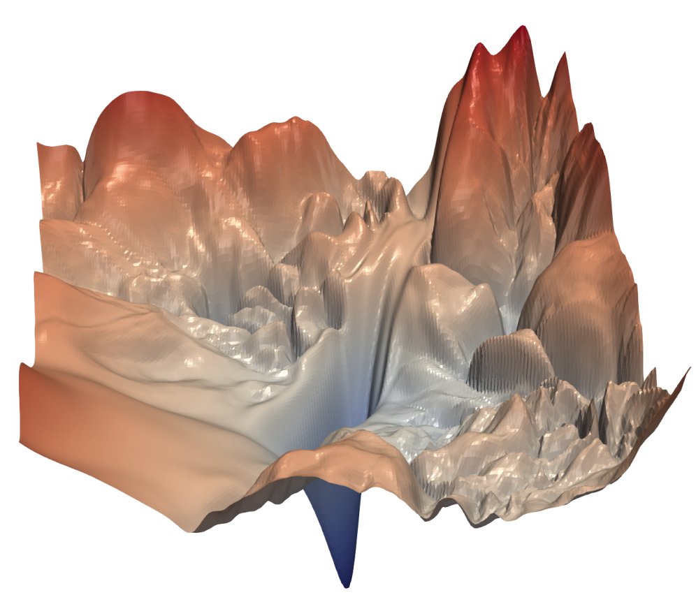
from Li et al
Project. Use a dimension reduction technique such as the singular value decomposition to visualize the loss surface of a neural network trained with MSE versus CE losses. The following is a possible outline:
- Start by training a neural network for a simple task. Perhaps to distinguish between
4s and9s. Save the vector of parameters at each optimization step together with the value of the loss function. - When training finishes you will have an matrix in \(\mathbb{R}^{p \times n}\) where \(p\) is the number of parameters in your model and \(n\) is the number of gradient steps you took in your training. Reduce dimension to create a matrix in \(\mathbb{R}^{2 \times n}\) whose rows can now be plotted against the values of the loss function.
- Augment your plot by adding more points not visited during your gradient descent. These have to be carefully chosen in \(\mathbb{R}^{p}\) and then projected only \(\mathbb{R}^2\).
- Now repeat the process using another loss function and compare the loss surfaces.
I have not seen this experiment done, but the results should be interesting and (presumably) support the heuristic that CE yields loss surfaces that are better suited for gradient-descent methods.